One of the toughest aspects of dealing with freeform data is that the input layer may not have proper data validation processes to ensure data cleanliness. This can result in very ugly records, including non-text fields that are riddled with incorrectly formatted values.
Take this example dataset:
[Test Data] table
RecordID
DurationField
1
00:24:00
2
00:22:56
3
00:54
4
0:30
5
01
6
4
7
2:44
8
5 MINUTES
9
6/19
Those values in the [DurationField] column are all different! How would we be able to consistently interpret this field as having a Interval data type?
One of the ways you might be inclined to handle something like this is to use If() statements. Let’s see an example of that now.
It’s a mess! Qlik has to evaluate each Interval#() function twice in order to, first, check to see if the value was properly interpreted as a duration (“interval”) value, and then, second, to actually return the interpreted duration value itself.
One of the nice alternative ways of handling this is to use a different conditional function, like Alt(). This function achieves the same thing as using the If() and IsNum() functions in conjunction. You can use:
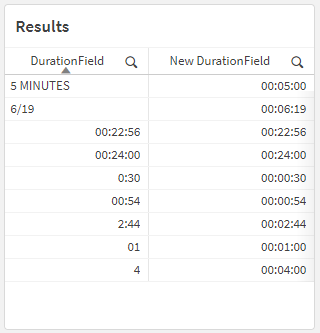
The preceding load happening at the bottom of that script is there to do some basic standardization of the [DurationField] field so that it’s easier to pattern-match.
In the rest of the script, we’re using the Alt() function (Qlik Help page) to check whether its arguments are numeric type of not. Each of its arguments are Interval#() functions, which are trying to interpret the values of the [DurationField] field as the provided format, like 'hh:mm:ss' or 'm:s'.
So it’s basically saying:
If Interval#([DurationField], 'hh:mm:ss') returns a value interpreted as an Interval, then return that value (for example, 00:24:00). But if a value couldn’t be interpreted as an Interval (like 5 mins for example, where the Interval#() function would return a text type), we go to the next Interval#() function. If Interval#([DurationField], 'mm:ss') returns a value…
This should all result in a table that looks like this:
In this post, I want to look at how to use a few of the built-in Qlik GeoAnalytics functions that will allow us to manipulate and aggregate geographic data.
Specifically, we are going to look at how to calculate a bounding box for several grouped geographic points, reformat the result, and then calculate the centroid of those bounding boxes. This can be a useful transformation step when our data has geographic coordinates that you need to have aggregated into a single, centered point for a particular grouping.
In our example, we have a small dataset with a few records pertaining to Florida locations. It includes coordinates for each Zip Code that is within the city of Brandon. Our goal is to take those four coordinates, aggregate them into a single, centered point, and then return that point in the correct format for displaying it in a Qlik map object.
Here’s our data, loaded from an Inline table:
[Data]:
Load * Inline [
State   ,   County          ,   City            ,   Zip     ,   Lat         ,   Long
FL      ,   Hillsborough    ,   Apollo Beach    ,   33572   ,   27.770687   ,   -82.399753
FL      ,   Hillsborough    ,   Brandon         ,   33508   ,   27.893594   ,   -82.273524
FL      ,   Hillsborough    ,   Brandon         ,   33509   ,   27.934039   ,   -82.302518
FL      ,   Hillsborough    ,   Brandon         ,   33510   ,   27.955670   ,   -82.300662
FL      ,   Hillsborough    ,   Brandon         ,   33511   ,   27.909390   ,   -82.292292
FL      ,   Hillsborough    ,   Sun City        ,   33586   ,   27.674490   ,   -82.480954
];
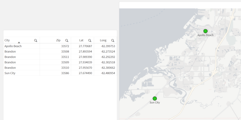
Let’s see what happens when we load this data and create a new map that has a point layer, using City as the dimension and the Lat/Long fields as the location fields:
What we may notice here is that the city of Brandon does not show up on the map — this is because the dimensional values for the point layer need to have only one possible location (in this case, one lat/long pair). Since Brandon has multiple Lat/Long pairs (one for each Zip Code), the map can’t display a single point for Brandon.
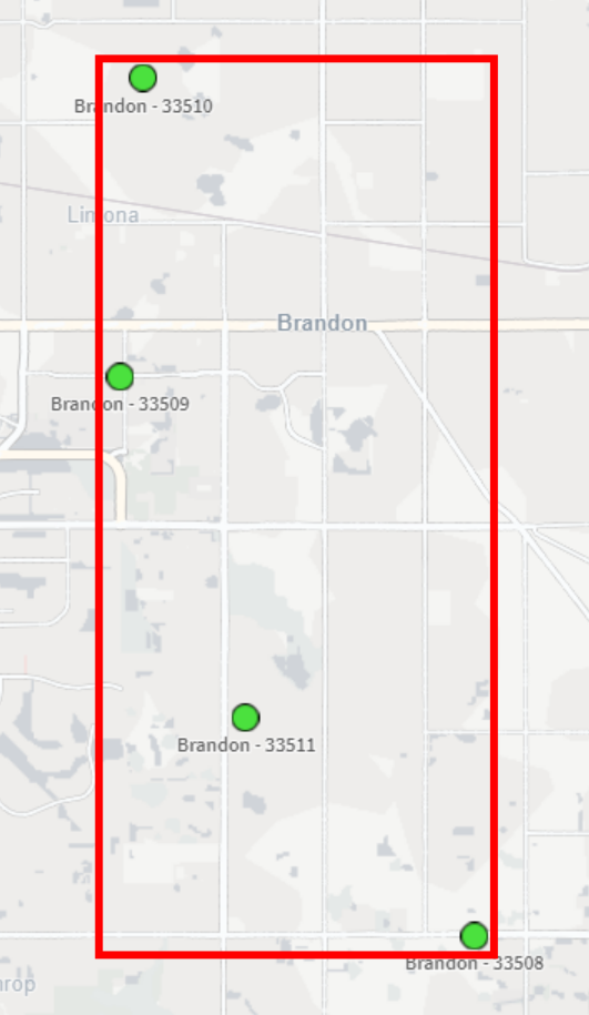
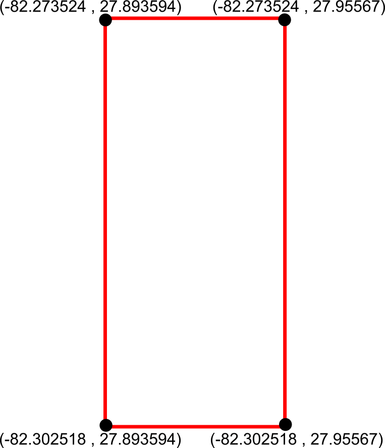
Okay, so let’s get the bounding box so that we can use it to get the center-most point. This is ultimately what we want our bounding box to be:
To do this in Qlik we’ll use the GeoBoundingBox() function, which calculates the smallest possible box that contains all given points, as shown in the example image above.
Here’s the script we can use in the Data Load Editor:
[Bounding Boxes]:
Load
    [City]
  , GeoBoundingBox('[' & Lat & ',' & Long & ']') as Box
Resident [Data]
  Group By [City]
;
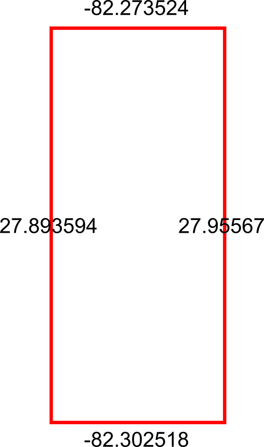
Alright so we now have our bounding boxes for our cities, but we can’t use those points quite yet — right now we just have the top, left, right, and bottom points separately:
What we need to do is reformat those points into actual coordinates for the bounding box, like so:
We can achieve this by using the JsonGet() function, which can return values for specific properties of a valid JSON string. This is useful to us because the GeoBoundingBox() function we used before returns the top, left, right, and bottom points in a JSON-like string that we can easily parse for this step.
Here’s the Qlik script we can use to parse those points into actual coordinates:
So now that we have these coordinates, we can aggregate the box coordinates into a center point using the GeoGetPolygonCenter() function, which will take the given area and output a centered point coordinate.
Here’s the script we can use for this:
[Centered Placenames]:
Load *
  , KeepChar(SubField([City Centroid], ',', 1), '0123456789.-') as [City Centroid Long]
  , KeepChar(SubField([City Centroid], ',', 2), '0123456789.-') as [City Centroid Lat]
;
Load
    [City]
  , GeoGetPolygonCenter([Box Formatted]) as [City Centroid]
Resident [Formatted Box];

Drop Table [Formatted Box];
This will result in the center points for each city. We also split out the Lat/Long fields into separate fields for easier use in the map:
City
City Centroid
City Centroid Lat
City Centroid Longitude
Apollo Beach
[-82.399753,27.770687]
27.770687
-82.399753
Brandon
[-82.288021,27.9094739069767]
27.9094739069767
-82.288021
Sun City
[-82.480954,27.67449]
27.67449
-82.480954
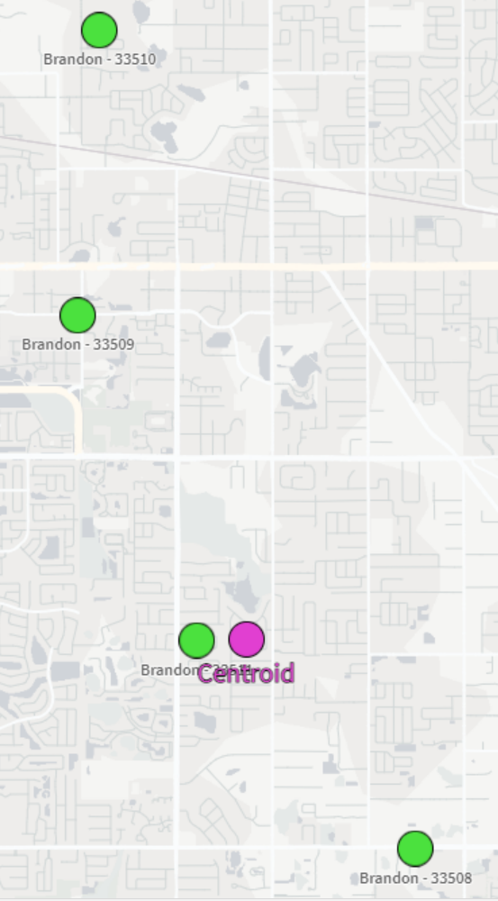
And now we can view our city-centered points on a map:
And there we have it! It’s not the perfect centering we may have expected but that could be due to the map projection that we’re using or the specificity of the coordinates we chose. Either way, this is a great way to be able to aggregate several coordinates down to their center point.
One of my biggest annoyances when it comes to cleaning data is needing to make a transformation that is seemingly super easy but turns out to be much more involved when it comes time to implement. I’ve found that while Qlik is not immune to these scenarios, you can very often script your way to a solution.
One of these common snafus is having to unpivot a table. Or…pivot it? Perhaps un-unpivot?
Let’s look at an example of how to pivot and then unpivot a table using Qlik script.
The Example
I first create a new app in Qlik Sense SaaS (though this all works exactly the same if using Qlik Sense on-prem). I am going to pull in the Raleigh Police Incidents (NIBRS) dataset, provided freely to the public via the city’s ArcGIS Open Data portal; here’s the link to the data:
Here’s our load script to bring in the table from a CSV file:
Notice the fields on lines 16-20 that begin with “reported” — these appear to be the same date field but with slightly different formats and granularity. Let’s check it out:
Just as we suspected. Now, what if we wanted to pivot (or “transpose”) those fields into just two fields: one for the field names and one for the field values? This can be done in either the Data Manager or the Data Load Editor. When scripting in the load editor, we use the Crosstable() function.
To do this, I’m going to choose to do this pivot with only the date fields and the unique ID field, which in this case is the [OBJECTID] field:
Our crosstable load looks like this:
This screenshot shows that, on lines 3-9, we are loading our key and date fields from the [Data] table we already loaded in. Then, on line 2, we use the Crosstable prefix and include 3 parameters:
[Date Field] is the field that will be created to hold the field names that appear on lines 4-9.
[Date Value] is the field that will be created to hold the field values from the fields on lines 4-9.
1 indicates that I only want to pivot the date fields around the first loaded field in this table, which is [OBJECTID] in this case. If this was 2, for example, then this operation would pivot the table around [OBJECTID] and [reported_date].
When we run this script, Qlik first loads the data from the CSV into the [Data] table, and then pivots (“crosstables”) the date fields around the key field, [OBJECTID], into a new table called [Dates].
We now see why we did this operation in a separate table and did not include all of the other fields – the pivot predictably increases the number of rows the app is now using:
Here’s what we now have:
Notice how the [Date Field] now holds all of those column names and the [Date Value] field now has those column values. We have successfully turned this:
…into this:
But what if our data had started out in a “pivoted” format? Or what if we want to simply unpivot that data?
The Solution
In order to unpivot the table, we’ll use a Generic Load and some clever scripting.
First, I’ll write the Generic Load:
This screenshot shows that I am using the [OBJECTID] field as my key, [Date Field] as the field names (“attributes”; these will be turned into separate columns), and [Date Value] as the field values (these will become the values for those separate columns).
Here’s the resulting schema:
We now have our data back in the column/value orientation we want, but we have an annoying issue: the resulting tables don’t auto-concatenate. We instead get a separate table for each unpivoted field.
Let’s write some script to always join these tables together without having to write a separate JOIN statement for each table:
Each line of this script is doing the following:
This line creates a new empty table called [Un-unpivoted] with only our key field, [OBJECTID].
*blank*
This line begins a For loop that starts with the number of loaded tables in our app up to this point (NoOfTables()-1) and then decrements (step -1) down to zero (to 0).
Here, inside the For loop, we set the variable vCurrentTable to the table name of the current loaded table index. This just means that every table loaded into the app at this point can be identified by the index at which they were loaded or joined. The first table loaded is 0, the next one is 1, etc. This order changes if that first table is joined with another table later on, though.
*blank*
Here, we check to see if the current table name begins with “Unpivoted.”, which is what our Generic Load tables are prepended with.
If the current table indeed begins with “Unpivoted.”, then we Resident the table with all of its fields and join it to the [Un-unpivoted] we created on line 1.
Now that we’ve joined our table into our master [Un-unpivoted] table, we can drop it from our data model.
This ends our IF statement.
This takes us to the next table index.
Here’s a table that shows the operations for each iteration:
Once we run this, we can see in the resulting table that we were successful!
About Blog
Arc Analytics is a full-service data analytics and integration consultancy based in Charlotte, NC, USA, specializing in the Qlik platform. Browse the posts below for practical Qlik tips, migration guidance, and real-world use cases from our consulting work.